GIS Concepts

Projections

A critical aspect of this project is the fact that numerous data layers over the entire political boundary of Ethiopia were used in the statistical analysis of this project, and also that the end goal of this project was to obtain density distribution maps which are inherently spatial.  Clearly then the need for all layers to be in the same projection was completely necessary for accuracy.  We chose to project all data in WGS 1984 37N projections as this was deemed to be the best available option given that our analysis was over all of Ethiopia (Newman, personal communication). 

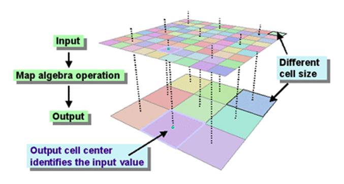
Resampling

It was necessary that the resolution of our data (cell size) were the same for all raster layers undergoing analysis.  Resampling is a method used in GIS that changes the proportions of a dataset by altering the cell size to achieve a specified resolution.  We chose the nearest neighbor sampling technique due to its applicability to both continuous and categorical data.  All raster datasets were resampled to a resolution of roughly 93 squared meters.

http://www.webhelp.esri.com

Figure 1. Left, resampling to a coarser resolution from a smaller resolution demonstrated in the input raster. Right, resampling from a rotated input raster, the cell center from the input raster closest to output raster's cell center is used.

To build and parameterize our model, it was necessary to sample a subset of points from the entire area of Ethiopia.  Samples needed to include a large number of points (large sample size) representative of all of Ethiopia’s regions populated by humans.  To achieve this we used the method of stratified sampling.  Stratified sampling is a method used to gain a representative sample from a large population when sub populations vary.  For example, we typically observe that population densities across the surface of a defined geographic area are not homogenous.  If points are sampled randomly without stratification, the majority of points will likely fall in areas that do not represent areas inhabited by a species of interest.  As a result, our abilities at making inferences are limited.  Stratifying groups into subgroups based on defined characteristics that those groups have in common (i.e. are they all spatially located close together, as in a city?) before sampling provides the ability to capture more of the variation that occurs in geographic space.  We chose Woredas (kind of like States) to stratify our random points in Ethiopia which as we believed confining a set number of points to each Woreda would provide insight into spatial correlations in the country.  For example, Woredas with large areas typically have lower population densities than those with small areas (which typically contain cities).  As a result, stratifying points to Woredsas provided a method to capture conditions that occur in areas with high population densities, and to capture conditions in less densely populated areas.  We used Hawth Tools (free extention for ESRI’s ArcGIS) to carry out stratified sampling.

Species Distributions

Niche modeling is an area of research in ecology that has received a tremendous amount of focus over the past decade.  It is also an area that is directly tied to geographic information systems (GIS) due to the spatial nature of a niche as defined by Grinnell (1917).  In niche modeling the goal is to measure environmental characteristics or attributes near the area where a species is observed.  These environmental variables can then be used to develop a predictive model based on numerous field observations (presences, absences, densities).  Before the advent of GIS spatial mapping of species distributions were not possible simply because the technology did not exist to implement such computationally intensive procedures.  Today, however, the GIS software is readily available to users and advanced analyses are very approachable even by nascent ecologists. 

Spatial Autocorrelation

Species distribution analyses often ignore the potential impacts of spatial autocorrelation.  Spatial autocorrelation occurs when two or more spatial variables correlate with each other through space (Liebhold and Sharov 1998).  For example, if one variable changes in one direction a second (or 3rd, 4th, etc.) will also change in that same direction.  It is not difficult to imagine situations where spatial autocorrelation should be addressed.  Consider a herd of bison or a rookery of seabirds.  Geographic information systems make it possible to address such issues, because these systems are inherently spatial.  Unfortunately the resolution of the density data for this project made it difficult to explicitly account for spatial autocorrelation.  Future studies will need to make efforts in this area and may consider using water features or road densities as a proxy for factors that could contribute to spatial autocorrelation, but it is unlikely that the limited availability of data for Ethiopia will allow this issue to be explicitly addressed until higher quality demographic data becomes available.

Spatial Climate Data

Climate data for this project was provided by WorldClim (Museum of Vertebrate Zoology, University of California, Berkeley).  Climate data from WorldClim was developed from precipitation records (47,554 locations), mean temperature (24,542 locations), and a range of temperatures (maximum and minimum, 14,835 locations).  Data were then interpolated using plate smoothing splines (Hijmans 2005) across the extent of the globe.  From this monthly data, bioclimatic variables determined to be biologically meaningful to many organisms and ecosystems were derived. These variables are frequently used in biological spatial niche modeling and represent trends, seasonality and factors that may be limiting to biological organisms.  The bioclimatic variables used in this project are provided below along with their coding.

BIO1 = Annual Mean Temperature
BIO2 = Mean Diurnal Range (Mean of monthly (max temp - min temp))
BIO3 = Isothermality (P2/P7) (* 100)
BIO4 = Temperature Seasonality (standard deviation *100)
BIO5 = Max Temperature of Warmest Month
BIO6 = Min Temperature of Coldest Month
BIO7 = Temperature Annual Range (P5-P6)
BIO8 = Mean Temperature of Wettest Quarter
BIO9 = Mean Temperature of Driest Quarter
BIO10 = Mean Temperature of Warmest Quarter
BIO11 = Mean Temperature of Coldest Quarter
BIO12 = Annual Precipitation
BIO13 = Precipitation of Wettest Month
BIO14 = Precipitation of Driest Month
BIO15 = Precipitation Seasonality (Coefficient of Variation)
BIO16 = Precipitation of Wettest Quarter
BIO17 = Precipitation of Driest Quarter
BIO18 = Precipitation of Warmest Quarter
BIO19 = Precipitation of Coldest Quarter

These variables are readily derived from min, max, and precipitation data available on WorldClim.  Some temperature values have been multiplied by 102 to preserve decimal places. An AML script is provided at the WorldClim website for BIOCLIM derivations.